Journal de mathématiques pures et appliquées de 1837
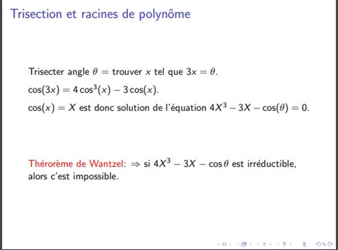
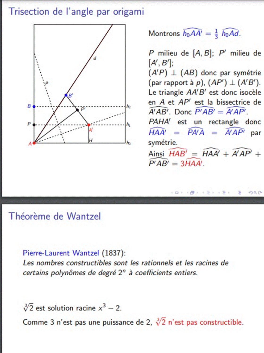
Texte établi par Joseph Liouville, 1837 (première série, tome 2, p. 369-375).
Recherches sur les moyens de reconnaître si un Problème de Géométrie peut se résoudre avec la règle et le compas ;
Par M. L. WANTZEL,
Élève-Ingénieur des Ponts-et-Chaussées.
I.
Supposons qu’un problème de Géométrie puisse être résolu par des intersections de lignes droites et de circonférences de cercles : si l’on joint les points ainsi obtenus avec les centres des cercles et avec les points qui déterminent les droites on formera un enchaînement de triangles rectilignes dont les éléments pourront être calculés par les formules de la Trigonométrie ; d’ailleurs ces formules sont des équations algébriques qui ne renferment les côtés et les lignes trigonométriques des angles qu’au premier et au second degré ; ainsi l’inconnue principale du problème s’obtiendra par la résolution d’une série d’équations du second degré dont les coefficients seront fonctions rationnelles des données de la question et des racines des équations précédentes. D’après cela, pour reconnaître si la construction d’un problème de Géométrie peut s’effectuer avec la règle et le compas, il faut chercher s’il est possible de faire dépendre les racines de l’équation à laquelle il conduit de celles d’un système d’équations du second degré composées comme on vient de l’indiquer. Nous traiterons seulement ici le cas où l’équation du problème est algébrique.
II.
Considérons la suite d’équations :
(A) {\displaystyle \left\{{\begin{alignedat}{2}x_{1}^{2}+{\rm {A}}x_{1}+{\rm {B}}=&0&x_{2}^{2}+{\rm {A_{1}}}x_{2}+{\rm {B_{1}}}=&0\ldots \\x_{n-1}^{2}+{\rm {A}}_{n-2}x_{n-1}+{\rm {B}}_{n-2}=&0&\qquad x_{n}^{2}+{\rm {A}}_{n-1}x_{n}+{\rm {B}}_{n-1}=&0\\\end{alignedat}}\right.}
{\displaystyle \left\{{\begin{alignedat}{2}x_{1}^{2}+{\rm {A}}x_{1}+{\rm {B}}=&0&x_{2}^{2}+{\rm {A_{1}}}x_{2}+{\rm {B_{1}}}=&0\ldots \\x_{n-1}^{2}+{\rm {A}}_{n-2}x_{n-1}+{\rm {B}}_{n-2}=&0&\qquad x_{n}^{2}+{\rm {A}}_{n-1}x_{n}+{\rm {B}}_{n-1}=&0\\\end{alignedat}}\right.}
 
dans lesquelles {\displaystyle {\rm {A}}}
{\rm {A}},{\displaystyle {\rm {B}}},p,{\displaystyle q},r,{\displaystyle {\rm {A_{1}}}},{\displaystyle {\rm {B_{1}}}},{\displaystyle x_{1},p,q},{\displaystyle {\rm {A_{m}}}},{\displaystyle {\rm {B_{m}}}},{\displaystyle x_{m},x_{m-1},\ldots ,x_{1},p,q\ldots }
 et {\displaystyle {\rm {B}}}
 représentent des fonctions rationnelles des quantités données {\displaystyle p}
, {\displaystyle q}
, {\displaystyle r}
… ; {\displaystyle {\rm {A_{1}}}}
 et {\displaystyle {\rm {B_{1}}}}
 des fonctions rationnelles de {\displaystyle x_{1},p,q}
, … ; et, en général, {\displaystyle {\rm {A_{m}}}}
 et {\displaystyle {\rm {B_{m}}}}
 des fonctions rationnelles de {\displaystyle x_{m},x_{m-1},\ldots ,x_{1},p,q\ldots }
Toute fonction rationnelle de {\displaystyle x_{m}}
{\displaystyle x_{m}} {\displaystyle {\rm {A_{m}}}} {\displaystyle {\rm {B_{m}}}} {\displaystyle {\frac {{\rm {C}}_{m-1}x_{m}+{\rm {D}}_{m-1}}{{\rm {E}}_{m-1}x_{m}+{\rm {F}}_{m-1}}}} {\displaystyle x_{m}}
 telle que {\displaystyle {\rm {A_{m}}}} ou {\displaystyle {\rm {B_{m}}}}, prend la forme {\displaystyle {\frac {{\rm {C}}_{m-1}x_{m}+{\rm {D}}_{m-1}}{{\rm {E}}_{m-1}x_{m}+{\rm {F}}_{m-1}}}} si l’on élimine les puissances de {\displaystyle x_{m}} supérieures à la pre
mière au moyen de l’équation {\displaystyle x_{m}^{2}+a_{m-1}x_{m}+{\rm {{B}_{m-1}=0}}}
{\displaystyle x_{m}^{2}+a_{m-1}x_{m}+{\rm {{B}_{m-1}=0}}},{\displaystyle {\rm {{C}_{m-1}}}},{\displaystyle {\rm {{E}_{m-1}}}},{\displaystyle {\rm {{F}_{m-1}}}},{\displaystyle x{m-1}},{\displaystyle x_{1}},p,{\displaystyle q},{\displaystyle {\rm {{A}_{m-1}^{\prime }x_{m}+{\rm {{B}_{m-1}^{\prime }}}}}}
, en désignant par {\displaystyle {\rm {{C}_{m-1}}}}
, {\displaystyle {\rm {{E}_{m-1}}}}
, {\displaystyle {\rm {{F}_{m-1}}}}
, des fonctions rationnelles de {\displaystyle x{m-1}}
, … {\displaystyle x_{1}}
, {\displaystyle p}
, {\displaystyle q}
… ; elle se ramènera ensuite à la forme {\displaystyle {\rm {{A}_{m-1}^{\prime }x_{m}+{\rm {{B}_{m-1}^{\prime }}}}}}
 en multipliant les deux termes de les deux termes de {\displaystyle {\frac {\rm {{C}_{m-1}x_{m}+{\rm {{D}_{m-1}}}}}{\rm {{E}_{m-1}x_{m}+{\rm {{F}_{m-1}}}}}}}
{\displaystyle {\frac {\rm {{C}_{m-1}x_{m}+{\rm {{D}_{m-1}}}}}{\rm {{E}_{m-1}x_{m}+{\rm {{F}_{m-1}}}}}}},{\displaystyle -{\rm {{E}_{m-1}({\rm {{A}_{m-1}+x_{m})}}}}},{\displaystyle +{\rm {{F}_{m-1}}}}
 par {\displaystyle -{\rm {{E}_{m-1}({\rm {{A}_{m-1}+x_{m})}}}}}
{\displaystyle +{\rm {{F}_{m-1}}}}
.
Multiplions l’une par l’autre les deux valeurs que prend le premier membre de la dernière des équations (A) lorsqu’on met successivement à la place de {\displaystyle x_{n-1}}
{\displaystyle x_{n-1}},{\displaystyle {\rm {{A}_{n-1}}}},{\displaystyle {\rm {{B}_{n-1}}}},{\displaystyle x_{n}},{\displaystyle x_{n-2},\ldots ,x_{1},p,q\ldots },{\displaystyle x_{n-2}},{\displaystyle x_{n}},{\displaystyle 2^{3}},{\displaystyle x_{n-3},\ldots ,x_{1},p,q,\ldots },{\displaystyle x_{n}},{\displaystyle 2^{n}},{\displaystyle p,q,r,\ldots .},{\displaystyle f(x_{n})=0},{\displaystyle f(x)=0}
 dans {\displaystyle {\rm {{A}_{n-1}}}}
 et {\displaystyle {\rm {{B}_{n-1}}}}
 les deux racines de l’équation précédente : nous aurons un polynôme du quatrième degré en {\displaystyle x_{n}}
 dont les coefficients s’exprimeront en fonction rationnelle de {\displaystyle x_{n-2},\ldots ,x_{1},p,q\ldots }
, remplaçons de même successivement dans ce polynôme {\displaystyle x_{n-2}}
 par les deux racines de l’équation correspondante, nous obtiendrons deux résultats dont le produit sera un polynôme en {\displaystyle x_{n}}
 de degré {\displaystyle 2^{3}}
, à coefficient rationnel par rapport à {\displaystyle x_{n-3},\ldots ,x_{1},p,q,\ldots }
 et, en continuant de la même manière, nous arriverons à un polynôme en {\displaystyle x_{n}}
 de degré {\displaystyle 2^{n}}
, dont les coefficients seront des fonctions rationnelles de {\displaystyle p,q,r,\ldots .}
 Ce polynôme égalé à zéro donnera l’équation finale {\displaystyle f(x_{n})=0}
 ou {\displaystyle f(x)=0}
, qui renferme toutes les solutions de la question. On peut toujours supposer qu’avant de faire le calcul on a réduit les équations (A) au plus petit nombre possible. Alors une quelconque d’entre elles {\displaystyle x_{m+1}^{2}+{\rm {{A}_{m}x_{m+1}+{\rm {{B}_{m}=0}}}}}
{\displaystyle x_{m+1}^{2}+{\rm {{A}_{m}x_{m+1}+{\rm {{B}_{m}=0}}}}}
, ne peut pas être satisfaite par une fonction rationnelle des quantités données et des racines des équations précédentes. Car, s’il en était ainsi, le résultat de la substitution serait une fonction rationnelle de {\displaystyle x_{m},\ldots ,x_{1},p,q,\ldots ,}
{\displaystyle x_{m},\ldots ,x_{1},p,q,\ldots ,},{\displaystyle {\rm {{A}'_{m-1}x_{m}+{\rm {{B}'_{m-1}\,}}}}},{\displaystyle {\rm {{A}'_{m-1}x_{m}+{\rm {{B}'_{m-1}=0\,}}}}},{\displaystyle x_{m}},{\displaystyle x_{m}},{\displaystyle {\rm {{A}'_{m-2}x_{m}+{\rm {{B}'_{m-2}=0\,}}}}},{\displaystyle {\rm {{A}'x_{1}+{\rm {{B}'=0\,}}}}},{\displaystyle x_{1}^{2}+{\rm {{A}x_{1}+{\rm {{B}=0}}}}},{\displaystyle p,q},{\displaystyle n-1}
 qu’on peut mettre sous la forme {\displaystyle {\rm {{A}'_{m-1}x_{m}+{\rm {{B}'_{m-1}\,}}}}}
 et l’on aurait {\displaystyle {\rm {{A}'_{m-1}x_{m}+{\rm {{B}'_{m-1}=0\,}}}}}
 ; on tirerait de cette relation une valeur rationnelle de {\displaystyle x_{m}}
 qui substituée dans l’équation du second degré en {\displaystyle x_{m}}
 conduirait à un résultat de la forme {\displaystyle {\rm {{A}'_{m-2}x_{m}+{\rm {{B}'_{m-2}=0\,}}}}}
. En continuant ainsi, on arriverait à {\displaystyle {\rm {{A}'x_{1}+{\rm {{B}'=0\,}}}}}
 ; c’est-à-dire que l’équation {\displaystyle x_{1}^{2}+{\rm {{A}x_{1}+{\rm {{B}=0}}}}}
 aurait pour racines des fonctions rationnelles de {\displaystyle p,q}
, … ; le système des équations (A) pourrait donc être remplacé par deux systèmes de {\displaystyle n-1}
 équations de second degré, indépendants l’un de l’autre, ce qui est contre la supposition. Si l’une des relations intermédiaires {\displaystyle {\rm {{A}'_{m-2}x_{m-1}+{\rm {{B}'_{m-2}=0\,}}}}}
{\displaystyle {\rm {{A}'_{m-2}x_{m-1}+{\rm {{B}'_{m-2}=0\,}}}}},{\displaystyle x_{m}^{2}+{\rm {{A}_{m-1}x_{m}+{\rm {{B}_{m-1}=0\,}}}}},{\displaystyle x_{m-1},\ldots ,x_{1}}
, par exemple, était satisfaite identiquement, les deux racines de l’équation {\displaystyle x_{m}^{2}+{\rm {{A}_{m-1}x_{m}+{\rm {{B}_{m-1}=0\,}}}}}
 seraient des fonctions rationnelles de {\displaystyle x_{m-1},\ldots ,x_{1}}
, pour toutes les valeurs que peuvent prendre ces quantités, en sorte qu’on pourrait supprimer l’équation
en {\displaystyle x_{m}}
{\displaystyle x_{m}}
 et remplacer la racine successivement par ses deux valeurs dans les équations sui
vantes, ce qui ramènerait encore le système des équations (A) à deux systèmes de {\displaystyle n-1}
{\displaystyle n-1}
 équations.
III.
Cela posé, l’équation du degré {\displaystyle 2^{n},f(x)=0}
{\displaystyle 2^{n},f(x)=0}
, qui donne toutes les solutions d’un problème susceptible d’être résolu au moyen de n équations du second degré, est nécessairement irréductible, c’est-à-dire qu’elle ne peut avoir de racines communes avec une équation de degré moindre dont les coefficients soient des fonctions rationnelles de données {\displaystyle p,q,\ldots .}
{\displaystyle p,q,\ldots .}
En effet, supposons qu’une équation {\displaystyle \operatorname {F} (x)=0,}
{\displaystyle \operatorname {F} (x)=0,},{\displaystyle x_{n}^{2}+{\rm {{A}_{n-1}x_{n}+{\rm {{B}_{n-1}=0}}}}},{\displaystyle x_{n-1},x_{n-2},\ldots ,x_{1}},{\displaystyle \operatorname {F} (x_{n}},{\displaystyle {\rm {{A}'_{n-1}x_{n}+{\rm {{B}'_{n-1}}}}}},{\displaystyle {\rm {{A}'_{n-1}}}},{\displaystyle {\rm {{B}'_{n-1}}}},{\displaystyle x_{n-1},\ldots ,x_{1},p,q,\ldots \,;},{\displaystyle {\rm {{A}'_{n-1}}}},{\displaystyle {\rm {{B}'_{n-1}}}},{\displaystyle {\rm {{A}'_{n-2}x_{n-1}+{\rm {{B}'_{n-2}}}}}},{\displaystyle {\rm {{A}'_{1}x_{2}+{\rm {{B}'_{1}}}}}},{\displaystyle {\rm {{A}'_{1}}}},{\displaystyle {\rm {{B}'_{1}}}},{\displaystyle {\rm {{A}'x_{1}+{\rm {{B}'}}}}},{\displaystyle {\rm {{A}'}}},{\displaystyle {\rm {{B}'}}},{\displaystyle p,q,\ldots .},{\displaystyle \operatorname {F} (x_{n})=0},{\displaystyle x_{n}},{\displaystyle {\rm {{A}'_{n-1}x_{n}+{\rm {{B}'_{n-1}=0}}}}},{\displaystyle {\rm {{A}'_{n-1}}}},{\displaystyle {\rm {{B}'_{n-1}}}}
 à coefficients rationnels soit satisfaite par une racine de l’équation {\displaystyle x_{n}^{2}+{\rm {{A}_{n-1}x_{n}+{\rm {{B}_{n-1}=0}}}}}
, en attribuant certaines valeurs convenables aux quantités {\displaystyle x_{n-1},x_{n-2},\ldots ,x_{1}}
. La fonction rationnelle {\displaystyle \operatorname {F} (x_{n}}
) d’une racine de cette dernière équation peut se ramener à la forme {\displaystyle {\rm {{A}'_{n-1}x_{n}+{\rm {{B}'_{n-1}}}}}}
, en désignant toujours par {\displaystyle {\rm {{A}'_{n-1}}}}
 et {\displaystyle {\rm {{B}'_{n-1}}}}
 des fonctions rationnelles de {\displaystyle x_{n-1},\ldots ,x_{1},p,q,\ldots \,;}
 de même {\displaystyle {\rm {{A}'_{n-1}}}}
 et {\displaystyle {\rm {{B}'_{n-1}}}}
 peuvent prendre l’une et l’autre la forme {\displaystyle {\rm {{A}'_{n-2}x_{n-1}+{\rm {{B}'_{n-2}}}}}}
, et ainsi de suite ; on arrivera ainsi à {\displaystyle {\rm {{A}'_{1}x_{2}+{\rm {{B}'_{1}}}}}}
, où {\displaystyle {\rm {{A}'_{1}}}}
 et {\displaystyle {\rm {{B}'_{1}}}}
 peuvent être mis sous la forme {\displaystyle {\rm {{A}'x_{1}+{\rm {{B}'}}}}}
, dans laquelle {\displaystyle {\rm {{A}'}}}
 et {\displaystyle {\rm {{B}'}}}
 représentent des fonctions rationnelles des données {\displaystyle p,q,\ldots .}
 Puisque {\displaystyle \operatorname {F} (x_{n})=0}
 pour une des valeurs de {\displaystyle x_{n}}
, on aura {\displaystyle {\rm {{A}'_{n-1}x_{n}+{\rm {{B}'_{n-1}=0}}}}}
, et il faudra que {\displaystyle {\rm {{A}'_{n-1}}}}
 et {\displaystyle {\rm {{B}'_{n-1}}}}
 soient nuls séparément, sans quoi l’équation {\displaystyle x_{n}^{2}+{\rm {{A}_{n-1}x_{n}+{\rm {{B}_{n-1}=0}}}}}
 serait satisfaite pour la valeur {\displaystyle {\frac {\rm {{B}'_{n-1}}}{\rm {{A}'_{n-1}}}}}
 qui est une fonction rationnelle de {\displaystyle x_{n-1},\ldots ,x_{1},p,q,\ldots \,;}
 ce qui est impossible ; de même, {\displaystyle {\rm {{A}'_{n-1}}}}
 et {\displaystyle {\rm {{B}'_{n-1}}}}
 étant nuls, {\displaystyle {\rm {{A}'_{n-2}}}}
 et {\displaystyle {\rm {{B}'_{n-2}}}}
 le seront aussi et ainsi de suite jusqu’à {\displaystyle {\rm {A'}}}
 et {\displaystyle {\rm {B'}}}
 qui seront nuls identiquement, puisqu’ils ne renferment que des quantités données. Mais alors {\displaystyle {\rm {{A}'_{1}}}}
 et {\displaystyle {\rm {{B}'_{1}}}}
, qui prennent également la forme {\displaystyle {\rm {{A}'x_{1}+{\rm {{B}'=0}}}}}
, quand on met pour {\displaystyle x_{1}}
 chacune des racines de l’équation {\displaystyle x_{1}^{2}+{\rm {{A}x_{1}+{\rm {{B}=0}}}}}
, s’annuleront pour ces deux valeurs
de {\displaystyle x_{1}}
{\displaystyle x_{1}} {\displaystyle {\rm {{A}'_{2}}}} {\displaystyle {\rm {{B}'_{2}}}} {\displaystyle {\rm {{A}'_{1}x_{2}+{\rm {{B}'_{1}}}}}} {\displaystyle x_{2}} {\displaystyle x_{2}^{2}+{\rm {{A}_{1}x_{2}+{\rm {{B}_{1}=0}}}}} {\displaystyle x_{1}} {\displaystyle x_{2}} {\displaystyle x_{1}} {\displaystyle {\rm {{A}'_{3}}}} {\displaystyle {\rm {{B}'_{3}}}} {\displaystyle x_{3}} {\displaystyle 2^{3}} {\displaystyle x_{2}} {\displaystyle x_{1}}
 ; pareillement, les coefficients {\displaystyle {\rm {{A}'_{2}}}} et {\displaystyle {\rm {{B}'_{2}}}} peuvent être mis sous la forme {\displaystyle {\rm {{A}'_{1}x_{2}+{\rm {{B}'_{1}}}}}} en prenant pour {\displaystyle x_{2}} l’une ou l’autre des racines de l’équation {\displaystyle x_{2}^{2}+{\rm {{A}_{1}x_{2}+{\rm {{B}_{1}=0}}}}}, correspondantes à chacune des valeurs de {\displaystyle x_{1}}, et par conséquent ils s’annuleront pour les quatre valeurs de {\displaystyle x_{2}} et pour les deux valeurs de {\displaystyle x_{1}} qui résultent de la combinaison des deux premières équations (A). On démontrera de même que {\displaystyle {\rm {{A}'_{3}}}} et {\displaystyle {\rm {{B}'_{3}}}} seront nuls en mettant pour {\displaystyle x_{3}} les {\displaystyle 2^{3}} valeurs tirées des trois premières équations (A) conjointement avec les valeurs correspondantes de {\displaystyle x_{2}} et {\displaystyle x_{1}} ;
et continuant de cette manière on conclura que {\displaystyle \operatorname {F} (x_{n})}
{\displaystyle \operatorname {F} (x_{n})},{\displaystyle 2^{n}},{\displaystyle x_{n}},{\displaystyle 2^{n}},{\displaystyle f(x)=0.},{\displaystyle \operatorname {F} (x)=0},{\displaystyle f(x)=0},{\displaystyle f(x)=0}
 s’annulera pour les {\displaystyle 2^{n}}
 valeurs de {\displaystyle x_{n}}
 auxquelles conduit le système de toutes les équations (A) ou pour les {\displaystyle 2^{n}}
 racines de {\displaystyle f(x)=0.}
 Ainsi une équation {\displaystyle \operatorname {F} (x)=0}
 à coefficients rationnels ne peut admettre une racine de {\displaystyle f(x)=0}
 sans les admettre toutes ; donc l’équation {\displaystyle f(x)=0}
 est irréductible.
IV.
Il résulte immédiatement du théorème précédent que tout problème qui conduit à une équation irréductible dont le degré n’est pas une puissance de {\displaystyle 2,}
{\displaystyle 2,},{\displaystyle x^{3}-2a^{3}=0}
 ne peut être résolu avec la ligne droite et le cercle. Ainsi la duplication du cube, qui dépend de l’équation {\displaystyle x^{3}-2a^{3}=0}
 toujours irréductible, ne peut être obtenue par la Géométrie élémentaire. Le problème des deux moyennes proportionnelles, qui conduit à l’équation {\displaystyle x^{3}-a^{2}b=0}
{\displaystyle x^{3}-a^{2}b=0},{\displaystyle b},a,{\displaystyle x^{3}-{\frac {3}{4}}x+{\frac {1}{4}}a=0\,;},a,a
 est dans le même cas toutes les fois que le rapport de {\displaystyle b}
 à {\displaystyle a}
 n’est pas un cube. La trisection de l’angle dépend de l’équation {\displaystyle x^{3}-{\frac {3}{4}}x+{\frac {1}{4}}a=0\,;}
 cette équation est irréductible si elle n’a pas de racine qui soit une fonction rationnelle de {\displaystyle a}
 et c’est ce qui arrive tant que {\displaystyle a}
 reste algébrique ; ainsi le problème ne peut être résolu en général avec la règle et le compas. Il nous semble qu’il n’avait pas encore été démontré rigoureusement que ces problèmes si célèbres chez les anciens, ne fussent pas susceptibles d’une solution par les constructions géométriques auxquelles ils s’attachaient particulièrement.
La division de la circonférence en parties égales peut toujours se ramener à la résolution de l’équation {\displaystyle x^{m}-1=0}
{\displaystyle x^{m}-1=0},m,m,{\displaystyle {\frac {x^{m}-1}{x-1}}=0},m-1
, dans laquelle {\displaystyle m}
 est un nombre premier ou une puissance d’un nombre premier. Lorsque {\displaystyle m}
 est premier, l’équation {\displaystyle {\frac {x^{m}-1}{x-1}}=0}
 du degré {\displaystyle m-1}
 est irréductible, comme M. Gauss l’a fait voir dans ses Disquisitiones arithmeticæ, section VII ; ainsi la division ne peut être effectuée par des constructions géométriques que si {\displaystyle m-1=2^{\alpha }}
{\displaystyle m-1=2^{\alpha }},m,{\displaystyle a^{\alpha }},{\displaystyle (a-1)a^{\alpha -1}},{\displaystyle x^{a^{\alpha }}-1},{\displaystyle x^{a^{\alpha -1}}-1},{\displaystyle (a-1)a^{\alpha -1}},{\displaystyle 2^{n}},{\displaystyle a-1,},{\displaystyle a=2.},{\displaystyle {\rm {N}}},{\displaystyle {\rm {N}}},2,{\displaystyle 2^{n}+1}
. Quand {\displaystyle m}
 est de la forme {\displaystyle a^{\alpha }}
, on peut prouver, en modifiant légèrement la démonstration de M. Gauss que l’équation de degré {\displaystyle (a-1)a^{\alpha -1}}
, obtenue en égalant à zéro le quotient de {\displaystyle x^{a^{\alpha }}-1}
 par {\displaystyle x^{a^{\alpha -1}}-1}
, est irréductible ; il faudrait donc que {\displaystyle (a-1)a^{\alpha -1}}
 fût de la forme {\displaystyle 2^{n}}
 en même temps que {\displaystyle a-1,}
 ce qui est impossible à moins que {\displaystyle a=2.}
 Ainsi, la division de la circonférence en {\displaystyle {\rm {N}}}
 parties ne peut être effectuée avec la règle et le compas que si les facteurs premiers de {\displaystyle {\rm {N}}}
 différents de {\displaystyle 2}
 sont de la forme {\displaystyle 2^{n}+1}
 et s’ils entrent seulement à la première puissance dans ce nombre. Ce principe est annoncé par M. Gauss à la fin de son ouvrage, mais il n’en a pas donné la démonstration.
Si l’on pose {\displaystyle x=k+{\rm {A}}'\,\,{\sqrt[{m'}]{a'}}+{\rm {A}}''\,\,{\sqrt[{m''}]{a''}}+\ldots }
{\displaystyle x=k+{\rm {A}}'\,\,{\sqrt[{m'}]{a'}}+{\rm {A}}''\,\,{\sqrt[{m''}]{a''}}+\ldots },m',{\displaystyle m''},{\displaystyle \ldots },2,k,{\displaystyle {\rm {A}}'},{\displaystyle {\rm {A}}''},{\displaystyle \ldots },{\displaystyle a'},{\displaystyle a''},{\displaystyle \ldots },x,x,m,{\displaystyle 2.},{\displaystyle x={\rm {A}}{\sqrt[{m}]{a}}},{\displaystyle ({\sqrt[{m}]{a}})^{p}},{\displaystyle p<m},x,m,{\displaystyle 2.}
, {\displaystyle m'}
, {\displaystyle m''}
, {\displaystyle \ldots }
, étant des puissances de {\displaystyle 2}
, et {\displaystyle k}
, {\displaystyle {\rm {A}}'}
, {\displaystyle {\rm {A}}''}
, {\displaystyle \ldots }
, {\displaystyle a'}
, {\displaystyle a''}
, {\displaystyle \ldots }
 des nombres commensurables, la valeur de {\displaystyle x}
 se construira par la ligne droite et le cercle, en sorte que {\displaystyle x}
 ne peut être racine d’une équation irréductible d’un degré {\displaystyle m}
 qui ne soit pas une puissance de {\displaystyle 2.}
 Par exemple, on ne peut avoir, {\displaystyle x={\rm {A}}{\sqrt[{m}]{a}}}
, si {\displaystyle ({\sqrt[{m}]{a}})^{p}}
 est irrationnel pour {\displaystyle p<m}
 ; on démontrerait facilement que {\displaystyle x}
 ne peut prendre cette valeur lors même que {\displaystyle m}
 serait une puissance de {\displaystyle 2.}
 Nous retrouvons ainsi plusieurs cas particuliers des théorèmes sur les nombres incommensurables que nous avons établis ailleurs[1].
V.
Supposons qu’un problème ait conduit à une équation de degré {\displaystyle 2^{n},\ \operatorname {F} (x)=0}
{\displaystyle 2^{n},\ \operatorname {F} (x)=0}
 et qu’on se soit assuré que cette équation est irréductible ; il s’agit de reconnaître si la solution peut s’obtenir au moyen d’une série d’équations du second degré.
Reprenons les équations (A) :
(A) {\displaystyle \left\{{\begin{alignedat}{2}x_{1}^{2}+{\rm {A}}x_{1}+{\rm {B=}}&\,0,&x_{2}^{2}+{\rm {A}}_{1}x_{2}+{\rm {B_{1}=}}&\,0\ldots ,\\x_{n-1}^{2}+{\rm {A}}_{n-2}x_{n-1}+{\rm {B}}_{n-2}=&\,0,\qquad &x_{n}^{2}+{\rm {A}}_{n-1}x_{n}+{\rm {B}}_{n-1}=&\,0\end{alignedat}}\right.}
{\displaystyle \left\{{\begin{alignedat}{2}x_{1}^{2}+{\rm {A}}x_{1}+{\rm {B=}}&\,0,&x_{2}^{2}+{\rm {A}}_{1}x_{2}+{\rm {B_{1}=}}&\,0\ldots ,\\x_{n-1}^{2}+{\rm {A}}_{n-2}x_{n-1}+{\rm {B}}_{n-2}=&\,0,\qquad &x_{n}^{2}+{\rm {A}}_{n-1}x_{n}+{\rm {B}}_{n-1}=&\,0\end{alignedat}}\right.}
 
Il faudra construire l’équation {\displaystyle f(x)=0}
{\displaystyle f(x)=0},{\displaystyle x_{n}},{\displaystyle \operatorname {F} (x)=0.},{\displaystyle {\rm {A}}_{n-1}},{\displaystyle {\rm {B}}_{n-1}},{\displaystyle a_{n-1}x_{n-1}+a'_{n-1},},{\displaystyle b_{n-1}x_{n-1}+b'_{n-1}},{\displaystyle x_{n-1}\,},{\displaystyle x_{n}},{\displaystyle a_{n-1}},{\displaystyle a''_{n-1}x_{n-2}+a_{n-1}^{'''}},{\displaystyle a'_{n-1}},{\displaystyle a_{n-1}^{IV}x_{n-2}+a_{n-1}^{V}},{\displaystyle b_{n-1}},{\displaystyle b''_{n-1}x_{n-2}+b_{n-1}^{'''}},{\displaystyle b'_{n-1}},{\displaystyle b_{n-1}^{IV}x_{n-2}+b_{n-1}^{V}},{\displaystyle {\rm {A}}_{n-2}},{\displaystyle {\rm {B}}_{n-2}},{\displaystyle a_{n-2}x_{n-2}+a'_{n-2}},{\displaystyle b_{n-2}x_{n-2}+b'_{n-2}},{\displaystyle x_{n-2}},{\displaystyle x_{n-2}^{2}+{\rm {A}}_{n-3}x_{n-2}+{\rm {B}}_{n-3}=0},{\displaystyle a_{n-1}},{\displaystyle a'_{n-1}},{\displaystyle a''_{n-1}},{\displaystyle \ldots },{\displaystyle b_{n-1}},{\displaystyle b'_{n-1}},{\displaystyle \ldots },{\displaystyle \operatorname {F} (x)=0}
, à coefficients rationnels, qui donne toutes les valeurs de {\displaystyle x_{n}}
 et l’identifier avec l’équation donnée {\displaystyle \operatorname {F} (x)=0.}
 Pour faire ce calcul on remarque que {\displaystyle {\rm {A}}_{n-1}}
 et {\displaystyle {\rm {B}}_{n-1}}
 se ramènent à la forme {\displaystyle a_{n-1}x_{n-1}+a'_{n-1},}
 et {\displaystyle b_{n-1}x_{n-1}+b'_{n-1}}
, en sorte que l’élimination de {\displaystyle x_{n-1}\,}
 entre les deux dernières équations (A) se fait immédiatement, ce qui donne une équation du quatrième degré en {\displaystyle x_{n}}
 ; on y remplacera ensuite {\displaystyle a_{n-1}}
 par {\displaystyle a''_{n-1}x_{n-2}+a_{n-1}^{'''}}
, {\displaystyle a'_{n-1}}
 par {\displaystyle a_{n-1}^{IV}x_{n-2}+a_{n-1}^{V}}
, {\displaystyle b_{n-1}}
 par {\displaystyle b''_{n-1}x_{n-2}+b_{n-1}^{'''}}
, {\displaystyle b'_{n-1}}
 par {\displaystyle b_{n-1}^{IV}x_{n-2}+b_{n-1}^{V}}
 et {\displaystyle {\rm {A}}_{n-2}}
, {\displaystyle {\rm {B}}_{n-2}}
 par {\displaystyle a_{n-2}x_{n-2}+a'_{n-2}}
, {\displaystyle b_{n-2}x_{n-2}+b'_{n-2}}
, puis on éliminera {\displaystyle x_{n-2}}
 entre l’équation du 4e degré déjà obtenue et l’équation {\displaystyle x_{n-2}^{2}+{\rm {A}}_{n-3}x_{n-2}+{\rm {B}}_{n-3}=0}
 ; et ainsi de suite. Les derniers termes des séries {\displaystyle a_{n-1}}
, {\displaystyle a'_{n-1}}
, {\displaystyle a''_{n-1}}
, {\displaystyle \ldots }
, {\displaystyle b_{n-1}}
, {\displaystyle b'_{n-1}}
, {\displaystyle \ldots }
, etc., doivent être des fonctions rationnelles des coefficients de {\displaystyle \operatorname {F} (x)=0}
 ; si l’on peut leur assigner des valeurs rationnelles qui satisfassent aux équations de condition obtenues en identifiant, on reproduira les équations (A) dont le système équivaut à l’équation
{\displaystyle \operatorname {F} (x)=0}
 ; si les conditions ne peuvent être vérifiées en donnant des valeurs rationnelles aux indéterminées introduites, le problème ne peut être ramené au second degré.
On peut simplifier ce procédé, en supposant que les racines de chacune des équations (A) donnent le dernier terme de la suivante ; ainsi, l’on peut prendre {\displaystyle {\rm {B}}_{n-1}}
{\displaystyle {\rm {B}}_{n-1}},{\displaystyle {\rm {B}}_{n-1}=b_{n-1}x_{n-1}+b'_{n-1}},{\displaystyle x_{n-1}={\frac {{\rm {B}}_{n-1}-b'_{n-1}}{b_{n-1}}}}
 pour l’inconnue de l’avant-dernière équation, puisque {\displaystyle {\rm {B}}_{n-1}=b_{n-1}x_{n-1}+b'_{n-1}}
 d’où {\displaystyle x_{n-1}={\frac {{\rm {B}}_{n-1}-b'_{n-1}}{b_{n-1}}}}
 ; de cette manière les éliminations se font plus rapidement et l’on introduit quatre quantités indéterminées dans l’équation du quatrième degré qui résulte de la première élimination, huit dans l’équation du huitième degré, etc., en sorte que les conditions obtenues en identifiant, sont en même nombre que les quantités à déterminer. Mais on écarte aussi à l’avance le cas où l’une des quantités telle que {\displaystyle b_{n-1}}
{\displaystyle b_{n-1}}
 serait nulle, et il faut étudier ce cas séparément.
Soit, par exemple, l’équation {\displaystyle x^{4}+px^{2}+qx+r=0}
{\displaystyle x^{4}+px^{2}+qx+r=0},{\displaystyle x_{1}^{2}+{\rm {A}}x_{1}+{\rm {B}}=0},{\displaystyle x^{2}+(ax_{1}+a')x+x_{1}=0},{\displaystyle x_{1}}
. Prenons de suite les équations du second degré sous la forme {\displaystyle x_{1}^{2}+{\rm {A}}x_{1}+{\rm {B}}=0}
 et {\displaystyle x^{2}+(ax_{1}+a')x+x_{1}=0}
 ; en éliminant {\displaystyle x_{1}}
 et identifiant, on aura,
{\displaystyle 2a_{1}-{\rm {A}}a=0}
{\displaystyle 2a_{1}-{\rm {A}}a=0},{\displaystyle a'^{2}+{\rm {A}}aa'-{\rm {A}}+a^{2}{\rm {B}}=p},{\displaystyle 2a{\rm {B}}-a'{\rm {A}}=q},{\displaystyle {\rm {B}}=r\,}
, {\displaystyle a'^{2}+{\rm {A}}aa'-{\rm {A}}+a^{2}{\rm {B}}=p}
, {\displaystyle 2a{\rm {B}}-a'{\rm {A}}=q}
, {\displaystyle {\rm {B}}=r\,}
,
d’où
{\displaystyle {\rm {B}}=r,\ \ a={\frac {2q}{4r-{\rm {A}}^{2}}},\ \ a'={\frac {{\rm {A}}q}{4r-{\rm {A}}^{2}}},\ \ {\rm {A}}^{3}+p{\rm {A}}^{2}-4r{\rm {A}}+q^{2}-4rp=0.}
Comme {\displaystyle {\rm {B}},a}
{\displaystyle {\rm {B}},a},{\displaystyle a'},{\displaystyle {\rm {A}},p,q,r,},{\displaystyle {\rm {A}}},{\displaystyle q=0,},p,{\displaystyle r,},{\displaystyle {\rm {A}}=-p}
 et {\displaystyle a'}
 sont exprimés rationnellement au moyen de {\displaystyle {\rm {A}},p,q,r,}
 il faut et il suffit que l’équation du troisième degré en {\displaystyle {\rm {A}}}
 ait pour racine une fonction rationnelle des données. La condition est toujours satisfaite quand {\displaystyle q=0,}
 quels que soient {\displaystyle p}
 et {\displaystyle r,}
 car {\displaystyle {\rm {A}}=-p}
 satisfait alors à la dernière équation.
En prenant {\displaystyle x_{1}}
{\displaystyle x_{1}}
 pour dernier terme de la deuxième équation du second degré, on a exclu le cas où ce terme serait indépendant de la racine de la première équation ; mais en le traitant directement, on ne trouve aucune solution de la question qui ne soit comprise dans les équations ci-dessus.
Ainsi, par un calcul plus ou moins long, on pourra toujours s’assurer si un problème donné est susceptible d’être résolu au moyen d’une série d’équations du second degré, pouvu qu’on sache reconnaître si une équation peut être satisfaite par une fonction rationnelle des données, et si elle est irréductible. Une équation de degré {\displaystyle n}
n,1,2,{\displaystyle \ldots },{\displaystyle {\frac {n}{2}}}
 sera irréductible lorsqu’en cherchant les diviseurs de son premier membre de degrés {\displaystyle 1}
, {\displaystyle 2}
, {\displaystyle \ldots }
, {\displaystyle {\frac {n}{2}}}
, on n’en trouve aucun dont les coefficients soient fonctions rationnelles des quantités données.
La question peut donc toujours être ramenée à rechercher si une équation algébrique {\displaystyle \operatorname {F} (x)=0}
{\displaystyle \operatorname {F} (x)=0}
 à une seule inconnue peut avoir pour racine une fonction de ce genre. Pour cela, il y a plusieurs cas à considérer. 1o Si les coefficients ne dépendent que de nombres donnés entiers ou fractionnaires, il suffira d’appliquer la méthode des racines commensurables. 2o Il peut arriver que les données représentées par les lettres {\displaystyle p}
p,{\displaystyle q},r
, {\displaystyle q}
, {\displaystyle r}
 soient susceptibles de prendre une infinité de valeurs, et que la condition cesse d’être remplie, comme quand elles désignent plusieurs lignes prises arbitrairement : alors, après avoir ramené l’équation {\displaystyle \operatorname {F} (x)=0}
{\displaystyle \operatorname {F} (x)=0},p,{\displaystyle q},r,{\displaystyle \ldots },x,{\displaystyle a_{m}p^{m}-a_{m-1}p^{m-1}+\ldots +a_{0}},{\displaystyle a_{m}},{\displaystyle a_{m-1}\ldots ,},x,{\displaystyle q}
 à une forme telle que ses coefficients soient des fractions entières de {\displaystyle p}
, {\displaystyle q}
, {\displaystyle r}
, {\displaystyle \ldots }
 et que celui du premier terme soit l’unité, on remplacera {\displaystyle x}
 par {\displaystyle a_{m}p^{m}-a_{m-1}p^{m-1}+\ldots +a_{0}}
, et l’on égalera à zéro les coefficients des différentes puissances dans le résultat ; les équations obtenues en {\displaystyle a_{m}}
, {\displaystyle a_{m-1}\ldots ,}
 seront traitées comme l’équation en {\displaystyle x}
, c’est-à-dire qu’on y remplacera ces quantités par des fonctions entières de {\displaystyle q}
, et ainsi de suite jusqu’à ce qu’ayant épuisé toutes les lettres on soit arrivé à des équations numériques qui rentreront dans le premier cas. 3o Lorsque les données sont des nombres irrationnels, ils doivent être racines d’équations algébriques qu’on peut supposer irréductibles ; dans ce cas, si l’on remplace {\displaystyle x}
x,{\displaystyle a_{m}p^{m}+a_{m-1}p^{m-1}+\ldots +a_{0}},{\displaystyle \operatorname {F} (x)=0},p,p,{\displaystyle a_{m}},{\displaystyle a_{m-1}},{\displaystyle \ldots },{\displaystyle \operatorname {F} (x)=0},m,p
 par {\displaystyle a_{m}p^{m}+a_{m-1}p^{m-1}+\ldots +a_{0}}
 dans {\displaystyle \operatorname {F} (x)=0}
, le premier membre de l’équation en {\displaystyle p}
, ainsi obtenue, devra être divisible par celui de l’équation irréductible dont le nombre {\displaystyle p}
 est racine ; en exprimant que cette division se fait exactement, on aboutit à des équations en {\displaystyle a_{m}}
, {\displaystyle a_{m-1}}
, {\displaystyle \ldots }
, que l’on traitera comme l’équation {\displaystyle \operatorname {F} (x)=0}
, jusqu’à ce que l’on parvienne à des équations numériques. On doit remarquer que {\displaystyle m}
 peut toujours être pris inférieur au degré de l’équation qui donne {\displaystyle p}
.
Ces procédés sont d’une application pénible en général, mais on peut les simplifier et obtenir des résultats plus précis dans certains cas très étendus, que nous étudierons spécialement.
https://www.researchgate.net/publication/238920600_Geometric_phase_in_the_causal_quantum_theories
About
156
Publications
16,272
Reads 
2,925
Citations
Introduction
Gonzalo G de Polavieja currently works at Champalimaud Neuroscience Program. Gonzalo does research at the boundary of collective behavior, Neuroscience and AI
Skills and Expertise
Brain
Neuroscience
Behavior
Behavioral Neuroscience
Behavioral Analysis
Artificial Intelligence
applied AI
Machine Learning
Research experience
July 2008 - July 2014
Spanish National Research Council
Madrid, Spain
Position
Group Leader
Publications
Publications (156)
Preprint
Full-text available
Feb 2021
We show that every finite semilattice can be represented as an atomized semilattice, an algebraic structure with additional elements (atoms) that extend the semilattice's partial order. Each atom maps to one subdirectly irreducible component, and the set of atoms forms a hypergraph that fully defines the semilattice. An atomization always exists an...
Article
Aug 2020
[...]
Social experiences greatly define subsequent social behavior. Lack of such experiences, especially during critical phases of development, can severely impede the ability to behave adequately in social contexts. To date, it is not well characterized how early-life social isolation leads to social deficits and impacts development. In many model speci...
Figure 1: Distances between centroids in MNIST-20. Example result from...,Figure 2: Distances between centroids in MNIST-20. (off-diagonal) Each...,Results MNIST-20 dataset,Results butterfly dataset. Model selection is the corrected centroid shift,data:image/png;base64,iVBORw0KGgoAAAANSUhEUgAAAAEAAAABCAYAAAAfFcSJAAAADUlEQVR42mN89OjNfwAJDwOxHEacwgAAAABJRU5ErkJggg==
Supervised dimensionality reduction by a Linear Discriminant Analysis on pre-trained CNN features
Preprint
Full-text available
Jun 2020
We explore the application of linear discriminant analysis (LDA) to the features obtained in different layers of pretrained deep convolutional neural networks (CNNs). The advantage of LDA compared to other techniques in dimensionality reduction is that it reduces dimensions while preserving the global structure of data, so distances in the low-dime...
FIGURE 2 | Modular structure of the policy network. (A)...,FIGURE 3 | Training makes reward to increase and group behavior to...,Environment parameters described in the methods.,data:image/png;base64,iVBORw0KGgoAAAANSUhEUgAAAAEAAAABCAYAAAAfFcSJAAAADUlEQVR42mN89OjNfwAJDwOxHEacwgAAAABJRU5ErkJggg==,data:image/png;base64,iVBORw0KGgoAAAANSUhEUgAAAAEAAAABCAYAAAAfFcSJAAAADUlEQVR42mN89OjNfwAJDwOxHEacwgAAAABJRU5ErkJggg==
Automated Discovery of Local Rules for Desired Collective-Level Behavior Through Reinforcement Learning
Article
Full-text available
Jun 2020
Complex global behavior patterns can emerge from very simple local interactions between many agents. However, no local interaction rules have been identified that generate some patterns observed in nature, for example the rotating balls, rotating tornadoes and the full-core rotating mills observed in fish collectives. Here we show that locally inte...
Figure S1: Social avoidance area measures in pairs of larvae. (A) Pairs...,Figure S3: Effects of CuSO 4 and control treatment of social avoidance...,data:image/png;base64,iVBORw0KGgoAAAANSUhEUgAAAAEAAAABCAYAAAAfFcSJAAAADUlEQVR42mN89OjNfwAJDwOxHEacwgAAAABJRU5ErkJggg==,data:image/png;base64,iVBORw0KGgoAAAANSUhEUgAAAAEAAAABCAYAAAAfFcSJAAAADUlEQVR42mN89OjNfwAJDwOxHEacwgAAAABJRU5ErkJggg==,data:image/png;base64,iVBORw0KGgoAAAANSUhEUgAAAAEAAAABCAYAAAAfFcSJAAAADUlEQVR42mN89OjNfwAJDwOxHEacwgAAAABJRU5ErkJggg==
Early-life social experience shapes social avoidance reactions in larval zebrafish
Preprint
Full-text available
mars-20
[...]
Social experiences greatly define successive social behavior. Lack of such experiences, especially during critical phases of development, can severely impede the ability to behave adequately in social contexts. To date it is not well characterized how early-life social isolation leads to social deficits and impacts development. In many model specie...
Fig 1. Deep-learning a model of collective behaviour. (A) Variables...,Fig 2. Properties of interaction between a pair of fish in the...,Fig 4. Ground-truth validation using simulated trajectories with known...,Fig 5. Weighting function: How a fish aggregates information from...,Fig 6. Relevant neighbours in the aggregation. A (Upper panel) Three...
Deep attention networks reveal the rules of collective motion in zebrafish
Article
Full-text available
sept-19
A variety of simple models has been proposed to understand the collective motion of animals. These models can be insightful but may lack important elements necessary to predict the motion of each individual in the collective. Adding more detail increases predictability but can make models too complex to be insightful. Here we report that deep atten...
Fig. 1. Virtual reality environment and experimental design. (A)...,Fig. 2. Reported sense of ownership and sense of agency scores and...,Fig. 3. Effect of movement and morphological incongruence in reported...,Fig. 4. Correlations of reported ownership scores. (A) Reported...,Fig. 5. Effect of incongruent movement in reported sense of ownership...
Active control as evidence in favor of sense of ownership in the moving Virtual Hand Illusion
Article
Full-text available
May 2019
The sense of ownership, the feeling that our body belongs to ourselves, relies on multiple sources of sensory information. Among these sources, the contribution of visuomotor information is still debated. We tested the effect of active control in the sense of ownership in the moving Virtual Hand Illusion. Participants reported sense of ownership an...
Tracking by identification in idtracker.ai
a, Graphical user interface....,Using idtracker.ai to study small and large animal groups
a, Two adult...,Training dataset of individual images
(a) Holding grid used to record...,Attack score over time for seven pairs of fish staged to fight
Each...
Correlation between the average distance to the center of the tank and...
idtracker.ai: Tracking all individuals in large collectives of unmarked animals
Article
Full-text available
Feb 2019
[...]
Understanding of animal collectives is limited by the ability to track each individual. We describe an algorithm and software that extract all trajectories from video, with high identification accuracy for collectives of up to 100 individuals. idtracker.ai uses two convolutional networks: one that detects when animals touch or cross and another for...
Fig 2. The effect of disagreement in initial individual estimates on...,Fig 3. How initial disagreement shifts the consensus group estimates...,Fig 4. Fits of different aggregation rules to the observed group...,data:image/png;base64,iVBORw0KGgoAAAANSUhEUgAAAAEAAAABCAYAAAAfFcSJAAAADUlEQVR42mN89OjNfwAJDwOxHEacwgAAAABJRU5ErkJggg==,data:image/png;base64,iVBORw0KGgoAAAANSUhEUgAAAAEAAAABCAYAAAAfFcSJAAAADUlEQVR42mN89OjNfwAJDwOxHEacwgAAAABJRU5ErkJggg==
Adolescents show collective intelligence which can be driven by a geometric mean rule of thumb
Article
Full-text available
sept-18
[...]
How effective groups are in making decisions is a long-standing question in studying human and animal behaviour. Despite the limited social and cognitive abilities of younger people, skills which are often required for collective intelligence, studies of group performance have been limited to adults. Using a simple task of estimating the number of...
Data
sept-18
[...]
The relationship between individual estimates before and after group discussion in Experiment 1. (PDF)
Data
sept-18
[...]
The effect of disagreement (range) in initial estimates on improving group estimates in Experiment 2. (PDF)
Data
sept-18
[...]
The effect of question order and treatment on the disagreement (range) of initial estimates in Experiment 2. (PDF)
Data
sept-18
[...]
Log-likelihood of simple aggregation rules, the noisy geometric mean model, and confidence intervals for frequencies of the aggregation rules using the noisy geometric mean model. (PDF)
Data
sept-18
[...]
The relationship between the range of initial estimates and estimates given by the group or calculated from initial estimates in Experiment 1. (PDF)
Data
sept-18
[...]
Fits of different aggregation rules to the observed data at various levels of added noise in Experiment 1. (PDF)
Data
sept-18
[...]
Distribution of individual initial estimates in Experiment 2. (PDF)
Data
sept-18
[...]
The effect of question order on the absolute error of (initial and group consensus) estimates in Experiment 2. (PDF)
Data
sept-18
[...]
The age distribution of participants in Experiment 1, correlations within groups, and distribution of individual initial estimates. (PDF)
Data
sept-18
[...]
The jars of sweets used in Experiment 1 and Experiment 2. (PDF)
Data
sept-18
[...]
The use and consequence of different aggregation rules for different thresholds that define groups as having a low or high range in Experiment 1. (PDF)
Data
sept-18
[...]
Correlations across treatments in the range of individual initial estimates per group. (PDF)
Data
sept-18
[...]
The relationship between participants’ self-rated confidence and error and the change in individuals estimates between stages. (PDF)
Data
sept-18
[...]
The distribution of the difference between the group estimate and the mean of initial estimates. (PDF)
Article
Full-text available
Aug 2018
Theoretical studies of ecosystem models have generally concluded that large numbers of species will not stably coexist if the species are all competing for the same limited set of resources. Here, we describe a simple multi-trait model of competition where the presence of N resources will lead to the stable coexistence of up to 2 N species. Our mo...
Data
Aug 2018
Figure 1: Deep-learning a model of collective behaviour. (A) Variables...,Figure 3: Alignment, attraction and repulsion zones depend on kinematic...,data:image/png;base64,iVBORw0KGgoAAAANSUhEUgAAAAEAAAABCAYAAAAfFcSJAAAADUlEQVR42mN89OjNfwAJDwOxHEacwgAAAABJRU5ErkJggg==,data:image/png;base64,iVBORw0KGgoAAAANSUhEUgAAAAEAAAABCAYAAAAfFcSJAAAADUlEQVR42mN89OjNfwAJDwOxHEacwgAAAABJRU5ErkJggg==,data:image/png;base64,iVBORw0KGgoAAAANSUhEUgAAAAEAAAABCAYAAAAfFcSJAAAADUlEQVR42mN89OjNfwAJDwOxHEacwgAAAABJRU5ErkJggg==
Aggregation rule in animal collectives dynamically changes between majority and minority influence
Preprint
Full-text available
Aug 2018
A variety of simple models has been proposed to understand the collective motion of animals. These models can be insightful but lack important elements necessary to predict the motion of each individual in the collective. Adding more detail increases predictability but can make models too complex to be insightful. Here we report that deep attention...
Data
Aug 2018
Data
Aug 2018
Article
Aug 2018
A new study on the zebrafish has discovered a population of forebrain neurons necessary for social orienting, providing a foundation for dissecting social brain networks in this powerful vertebrate model.
Article
Full-text available
Aug 2018
Most animals fight by repeating complex stereotypic behaviours, yet the internal structure of these behaviours has rarely been dissected in detail. We characterized the internal structure of fighting behaviours by developing a machine learning pipeline that measures and classifies the behaviour of individual unmarked animals on a sub-second time sc...
Figure 1: Training the network. Left panel: sample images from the...,data:image/png;base64,iVBORw0KGgoAAAANSUhEUgAAAAEAAAABCAYAAAAfFcSJAAAADUlEQVR42mN89OjNfwAJDwOxHEacwgAAAABJRU5ErkJggg==,data:image/png;base64,iVBORw0KGgoAAAANSUhEUgAAAAEAAAABCAYAAAAfFcSJAAAADUlEQVR42mN89OjNfwAJDwOxHEacwgAAAABJRU5ErkJggg==,data:image/png;base64,iVBORw0KGgoAAAANSUhEUgAAAAEAAAABCAYAAAAfFcSJAAAADUlEQVR42mN89OjNfwAJDwOxHEacwgAAAABJRU5ErkJggg==,data:image/png;base64,iVBORw0KGgoAAAANSUhEUgAAAAEAAAABCAYAAAAfFcSJAAAADUlEQVR42mN89OjNfwAJDwOxHEacwgAAAABJRU5ErkJggg==
Sensory cheating: adversarial body patterns can fool a convolutional visual system during signaling
Preprint
Full-text available
May 2018
Animals often assess each other by paying special attention to signals, which help to communicate the quality of each individual. When there is a conflict of interest between the signaler and the receiver, then the signaler has an incentive to cheat by producing signals which exaggerate its apparent quality. One opportunity for cheating might be to...
Table 3 : Sixth-Order Kernels ,Behavioral inter-individual variability in a population of 48 larval...,Impact of environmental changes and genetic background on behavioral...,Epigenetic modulation of behavioral inter-individual variability. a...
Relation between histone acetylation levels and behavior. a Average...
Histone H4 acetylation regulates behavioral inter-individual variability in zebrafish
Article
Full-text available
Apr 2018
[...]
Background: Animals can show very different behaviors even in isogenic populations, but the underlying mechanisms to generate this variability remain elusive. We use the zebrafish (Danio rerio) as a model to test the influence of histone modifications on behavior. Results: We find that laboratory and isogenic zebrafish larvae show consistent ind...
Data
Apr 2018
[...]
Data
Apr 2018
[...]
Figure 4: Testing the relationship between compression and error rate...,Figure 5: Learning to distinguish one hand-written digit from the rest....,Figure 6: Atoms in digit recognition. Example atoms in the training for...,Figure 7: Agreement of 10 master atomizations. Top: Count of the number...
Figure 8: False positive and negative ratios using multiple master...
Algebraic Machine Learning
Article
Full-text available
mars-18
Machine learning algorithms use error function minimization to fit a large set of parameters in a preexisting model. However, error minimization eventually leads to a memorization of the training dataset, losing the ability to generalize to other datasets. To achieve generalization something else is needed, for example a regularization method or st...
Figure 1: Tracking by identiication in idtracker.ai. a. Graphical user...,Architectures with variations in the number of convolutional lay- ers...,data:image/png;base64,iVBORw0KGgoAAAANSUhEUgAAAAEAAAABCAYAAAAfFcSJAAAADUlEQVR42mN89OjNfwAJDwOxHEacwgAAAABJRU5ErkJggg==,data:image/png;base64,iVBORw0KGgoAAAANSUhEUgAAAAEAAAABCAYAAAAfFcSJAAAADUlEQVR42mN89OjNfwAJDwOxHEacwgAAAABJRU5ErkJggg==,data:image/png;base64,iVBORw0KGgoAAAANSUhEUgAAAAEAAAABCAYAAAAfFcSJAAAADUlEQVR42mN89OjNfwAJDwOxHEacwgAAAABJRU5ErkJggg==
idtracker.ai: Tracking all individuals in large collectives of unmarked animals
Preprint
Full-text available
mars-18
[...]
Our understanding of collective animal behavior is limited by our ability to track each of the individuals. We describe an algorithm and software, idtracker.ai, that extracts from video all trajectories with correct identities at a high accuracy for collectives of up to 100 individuals. It uses two deep networks, one detecting when animals touch or...
Decision-making in collectives with re-evaluation of choice. a Simple...,Re-evaluation implies the highest accuracy at intermediate group size....,Error propagation in large groups. a Probability that the first...,Accuracy for different decision rules. a Examples of individual...
Different degrees of randomness in decision order. Results for decision...
Dynamic choices are most accurate in small groups
Article
Full-text available
mars-18
According to the classic results of Galton and Condorcet, as well as in modern decision-making models, accuracy in groups increases with group size. However, these studies do not consider the naturally occurring situation in which individuals dynamically re-evaluate their decision with a possible change of opinion. The dynamics of re-evaluation in...
Figure 1: Species abundance distributions (SADs). SADs for two...,Figure 2: Simulation of removal experiments. The blue points plot the...,Figure 3: The analytical formula in Equation (1) gives a good...,data:image/png;base64,iVBORw0KGgoAAAANSUhEUgAAAAEAAAABCAYAAAAfFcSJAAAADUlEQVR42mN89OjNfwAJDwOxHEacwgAAAABJRU5ErkJggg==,data:image/png;base64,iVBORw0KGgoAAAANSUhEUgAAAAEAAAABCAYAAAAfFcSJAAAADUlEQVR42mN89OjNfwAJDwOxHEacwgAAAABJRU5ErkJggg==
Towards a unification of niche and neutral models of community ecology
Preprint
Full-text available
Feb 2018
Ecological models of community dynamics fall into two main categories. The neutral theory of biodiversity correctly predicts various large-scale ecosystem characteristics such as the species abundance distributions. On a smaller scale, the niche theory of species competition explains population dynamics and interactions between two to a dozen speci...
Figure 2: A kinematic characterization of a fight. A: The fraction of...,Figure 3: Forcemaps of the defender in the symmetric (top row) and...,data:image/png;base64,iVBORw0KGgoAAAANSUhEUgAAAAEAAAABCAYAAAAfFcSJAAAADUlEQVR42mN89OjNfwAJDwOxHEacwgAAAABJRU5ErkJggg==,data:image/png;base64,iVBORw0KGgoAAAANSUhEUgAAAAEAAAABCAYAAAAfFcSJAAAADUlEQVR42mN89OjNfwAJDwOxHEacwgAAAABJRU5ErkJggg==,data:image/png;base64,iVBORw0KGgoAAAANSUhEUgAAAAEAAAABCAYAAAAfFcSJAAAADUlEQVR42mN89OjNfwAJDwOxHEacwgAAAABJRU5ErkJggg==
Characterizing the sub-second timescale strategies of fighting in zebrafish
Preprint
Full-text available
Dec 2017
Most animals fight by repeating complex stereotypic behaviors, yet the internal structure of these behaviors has rarely been dissected in detail. We characterized the internal structure of fighting behaviors by developing a machine learning pipeline that measures and classifies the behavior of individual unmarked animals on a sub-second timescale....
FIGURE 1 | The three factors that influence aggregation rules. (A-C):...,FIGURE 3 | Following the informed minority vs. majority voting. The red...,FIGURE 4 | Wisdom of the crowd for historical dates. Mean of 50...,FIGURE 5 | Comparison of averaging and choosing strategies for...
FIGURE 6 | Errors in human advice-taking strategy compared to the...
Rescuing Collective Wisdom when the Average Group Opinion Is Wrong
Article
Full-text available
nov-17
The total knowledge contained within a collective supersedes the knowledge of even its most intelligent member. Yet the collective knowledge will remain inaccessible to us unless we are able to find efficient knowledge aggregation methods that produce reliable decisions based on the behavior or opinions of the collective’s members. It is often stat...
Article
Full-text available
nov-17
Decision-making theories explain animal behaviour, including human behaviour, as a response to estimations about the environment. In the case of collective behaviour, they have given quantitative predictions of how animals follow the majority option. However, they have so far failed to explain that in some species and contexts social cohesion incre...
Data
nov-17
Data
sept-17
[...]
Simulated voltage responses of a biophysically realistic R1-R6 photoreceptor model to very bright 20 Hz, 50 Hz, 100 Hz, 200 Hz and 500 Hz GWN light stimuli at BG1.
Data
sept-17
[...]
Intracellular voltage responses of the same R1-R6 photoreceptor to very bright 20 Hz, 50 Hz, 100 Hz, 200 Hz and 500 Hz bursty light stimuli at BG0 (darkness).
Data
sept-17
[...]
Intracellular voltage responses of the same R1-R6 photoreceptor to very bright 20 Hz, 50 Hz, 100 Hz, 200 Hz and 500 Hz bursty light stimuli at BG0.5.
Data
sept-17
[...]
Simulated voltage responses of a biophysically realistic R1-R6 photoreceptor model to very bright 20 Hz, 50 Hz, 100 Hz, 200 Hz and 500 Hz bursty light stimuli at BG0.5.
Data
sept-17
[...]
Intracellular voltage responses of the same R1-R6 photoreceptor to very bright 20 Hz, 50 Hz, 100 Hz, 200 Hz and 500 Hz bursty light stimuli at BG1.
Data
sept-17
[...]
Intracellular voltage responses of the same R1-R6 photoreceptor to very bright 20 Hz, 50 Hz, 100 Hz, 200 Hz and 500 Hz bursty light stimuli at BG1.5.
Data
sept-17
[...]
Simulated voltage responses of a biophysically realistic R1-R6 photoreceptor model to very bright 20 Hz, 50 Hz, 100 Hz, 200 Hz and 500 Hz bursty light stimuli at BG0 (darkness).
Data
sept-17
[...]
Simulated voltage responses of a biophysically realistic R1-R6 photoreceptor model to very bright 20 Hz, 50 Hz, 100 Hz, 200 Hz and 500 Hz GWN light stimuli at BG1.5.
Article
Full-text available
sept-17
[...]
Article
sept-17
Insects are capable of spectacular achievements through collective behavior, but examples of such behavior in fruit flies are rare. New research indicates that Drosophila larvae engage in coordinated digging to feed collectively.
Preprint
Aug 2017
[...]
Animals can show very different behaviors even in isogenic populations, but the underlying mechanisms to generate this variability remain elusive. We found that laboratory and isogenic zebrafish ( Danio rerio ) larvae showed consistent individual behaviors when swimming freely in identical wells or in reaction to stimuli. We also found that this be...
Figure 1. Photoreceptors respond best to highcontrast bursts. (A)...,Figure 1-figure supplement 1. R1-R6 output varies more cell-to-cell...,Figure 2. High-contrast bursts drive maximal encoding. A R1-R6's...,Figure 2-figure supplement 1. Signaling performance vary cell-to-cell...
Figure 2-figure supplement 2. Light-adapted R1-R6 noise is similar for...
Microsaccadic sampling of moving image information provides Drosophila hyperacute vision
Preprint
Full-text available
Jul 2017
[...]
Small fly eyes should not see fine image details. Because flies exhibit saccadic visual behaviors and their compound eyes have relatively few ommatidia (sampling points), their photoreceptors would be expected to generate blurry and coarse retinal images of the world. Here we demonstrate that Drosophila see the world far better than predicted from...
Figure 1-figure supplement 1. R1-R6 output varies more cell-to-cell...,Figure 2-Figure supplement 4. Drosophila R1-R6 photoreceptor output...,Figure 2-figure supplement 1. Signaling performance vary cell-to-cell...,Figure 2-figure supplement 3. Strong responses to naturalistic...
Figure 2. High-contrast bursts drive maximal encoding. A R1-R6's...
Microsaccadic sampling of moving image information provides Drosophila hyperacute vision
Article
Full-text available
Jul 2017
[...]
Small fly eyes should not see fine image details. Because flies exhibit saccadic visual behaviors and their compound eyes have relatively few ommatidia (sampling points), their photoreceptors would be expected to generate blurry and coarse retinal images of the world. Here we demonstrate that Drosophila see the world far better than predicted from...
Article
Full-text available
Apr 2017
Animals moving in groups coordinate their motion to remain cohesive. A large amount of data and analysis of movement coordination has been obtained in several species, but we are lacking theoretical frameworks that can derive the form of coordination rules. Here, we examine whether optimal control theory can predict the rules underlying social inte...
Data
Apr 2017
Article
Apr 2017
A great challenge in neuroscience is understanding how activity in the brain gives rise to behavior. The zebrafish is an ideal vertebrate model to address this challenge, thanks to the capacity, at the larval stage, for precise behavioral measurements, genetic manipulations, and recording and manipulation of neural activity noninvasively and at sin...
Figure 1 The accuracy of the first approach significantly increased...,Figure 2 (a) After making an incorrect initial approach, we found that...,data:image/png;base64,iVBORw0KGgoAAAANSUhEUgAAAAEAAAABCAYAAAAfFcSJAAAADUlEQVR42mN89OjNfwAJDwOxHEacwgAAAABJRU5ErkJggg==,data:image/png;base64,iVBORw0KGgoAAAANSUhEUgAAAAEAAAABCAYAAAAfFcSJAAAADUlEQVR42mN89OjNfwAJDwOxHEacwgAAAABJRU5ErkJggg==,data:image/png;base64,iVBORw0KGgoAAAANSUhEUgAAAAEAAAABCAYAAAAfFcSJAAAADUlEQVR42mN89OjNfwAJDwOxHEacwgAAAABJRU5ErkJggg==
Collective decision making in guppies: A cross-population comparison study in the wild
Article
Full-text available
Feb 2017
[...]
Collective cognition has received much attention in recent years but most of the empirical work has focused on comparing individuals and groups within single populations, thereby not addressing evolutionary origins of collective cognition. Here, we investigated collective cognition in multiple populations that are subject to different levels of pre...
Fig. 3. Development of attraction. (A) Probability of accelerating...,Fig. 4. Attraction rule from developmental data. (A) Diagram of model...,Fig. 5. Aggregation from agent-based simulations. (A) Most likely...,data:image/png;base64,iVBORw0KGgoAAAANSUhEUgAAAAEAAAABCAYAAAAfFcSJAAAADUlEQVR42mN89OjNfwAJDwOxHEacwgAAAABJRU5ErkJggg==,data:image/png;base64,iVBORw0KGgoAAAANSUhEUgAAAAEAAAABCAYAAAAfFcSJAAAADUlEQVR42mN89OjNfwAJDwOxHEacwgAAAABJRU5ErkJggg==
Ontogeny of collective behavior reveals a simple attraction rule
Article
Full-text available
Feb 2017
The striking patterns of collective animal behavior, including ant trails, bird flocks, and fish schools, can result from local interactions among animals without centralized control. Several of these rules of interaction have been proposed, but it has proven difficult to discriminate which ones are implemented in nature. As a method to better disc...
Article
janv-17
Evolutionary game theory has been the theoretical tool of choice for analysis of social interactions in general and aggressive interaction in particular. Many important game theory models of aggression are formulated based on assumptions about short timescale behavior but are tested trough measuring long timescale behavior. The resulting methodolog...
TABLE 1 | Summary of the neuropathological conditions affecting...,data:image/png;base64,iVBORw0KGgoAAAANSUhEUgAAAAEAAAABCAYAAAAfFcSJAAAADUlEQVR42mN89OjNfwAJDwOxHEacwgAAAABJRU5ErkJggg==,data:image/png;base64,iVBORw0KGgoAAAANSUhEUgAAAAEAAAABCAYAAAAfFcSJAAAADUlEQVR42mN89OjNfwAJDwOxHEacwgAAAABJRU5ErkJggg==,data:image/png;base64,iVBORw0KGgoAAAANSUhEUgAAAAEAAAABCAYAAAAfFcSJAAAADUlEQVR42mN89OjNfwAJDwOxHEacwgAAAABJRU5ErkJggg==,data:image/png;base64,iVBORw0KGgoAAAANSUhEUgAAAAEAAAABCAYAAAAfFcSJAAAADUlEQVR42mN89OjNfwAJDwOxHEacwgAAAABJRU5ErkJggg==
Toward a Molecular Profile of Self-Representation
Article
Full-text available
nov-16
Feeling embodiment over our body or body part has a major role in the understanding of the self and control of self-actions. Even though it is crucial in our daily life, embodiment is not an homogenous phenotype across population, as quantified by implicit and explicit measures (i.e., neuroimaging or self-reports). Studies have shown differences in...
Data
nov-16
[...]
Electronic Supplementary Material: Details of fish rearing conditions and three Supplementary Figures (Figures S1-S3) are provided
https://www.researchgate.net/profile/Andrew-King-11/publication/310614981/figure/fig1/AS:613891063164937@1523374443682/figure-fig1_Q320.jpg,data:image/png;base64,iVBORw0KGgoAAAANSUhEUgAAAAEAAAABCAYAAAAfFcSJAAAADUlEQVR42mN89OjNfwAJDwOxHEacwgAAAABJRU5ErkJggg==,data:image/png;base64,iVBORw0KGgoAAAANSUhEUgAAAAEAAAABCAYAAAAfFcSJAAAADUlEQVR42mN89OjNfwAJDwOxHEacwgAAAABJRU5ErkJggg==,data:image/png;base64,iVBORw0KGgoAAAANSUhEUgAAAAEAAAABCAYAAAAfFcSJAAAADUlEQVR42mN89OjNfwAJDwOxHEacwgAAAABJRU5ErkJggg==,data:image/png;base64,iVBORw0KGgoAAAANSUhEUgAAAAEAAAABCAYAAAAfFcSJAAAADUlEQVR42mN89OjNfwAJDwOxHEacwgAAAABJRU5ErkJggg==
European sea bass show behavioural resilience to near-future ocean acidification
Article
Full-text available
nov-16
[...]
Ocean acidification (OA)-caused by rising concentrations of carbon dioxide (CO2)-is thought to be a major threat to marine ecosystems and has been shown to induce behavioural alterations in fish. Here we show behavioural resilience to nearfuture OA in a commercially important and migratory marine finfish, the Sea bass (Dicentrarchus labrax). Sea ba...
Article
Jul 2016
[...]
Doublecortin (DCX)-Calretinin (CLR) immunolabeling of the hippocampal dentate gyrus of a 4 month old male mice (Mus musculus). DCX+ (red) and CLR+ (green) neurons in a section from a control (no treatment) mouse, where both DCX+/CLR+ and DCX+/CLR+ can be appreciated. This dual labeling lets to count two different subpopulation of immature, differen...
Preprint
Jul 2016
In adverse conditions, individuals follow the majority more strongly. This phenomenon is very general across social species, but explanations have been particular to the species and context, including antipredatory responses, deflection of responsibility, or increase in uncertainty. Here we show that the impact of social information in realistic de...
Article
janv-16
[...]
The influence of the learning process on the persistence of the newly acquired behavior is relevant both for our knowledge of the learning/memory mechanisms and for the educational policy. However, it is unclear whether during an operant conditioning process with a continuous reinforcement paradigm, individual differences in acquisition are also as...
Article
Full-text available
janv-16
[...]
Ocean acidification (OA)—caused by rising concentrations of carbon dioxide (CO2)—is thought to be a major threat to marine ecosystems and has been shown to induce behavioural alterations in fish. Here we show behavioural resilience to near-future OA in a commercially important migratory marine finfish, the European sea bass (Dicentrarchus labrax)....
Figure S1. Data-processing and error elimination. Example of erroneous...,Figure S2. Example of a single fish's trajectory and the corresponding...,Figure S2. Example of a single fish's trajectory and the corresponding...,Figure S3 Comparison of speed and movement data from real fish and...,data:image/png;base64,iVBORw0KGgoAAAANSUhEUgAAAAEAAAABCAYAAAAfFcSJAAAADUlEQVR42mN89OjNfwAJDwOxHEacwgAAAABJRU5ErkJggg==
Electronic Supplementary Material%3A Details of fish rearing conditions and three Supplementary Figures (Figures S1-S3) are provided from European sea bass show behavioural resilience to near-future ocean acidification
Article
Full-text available
janv-16
[...]
Ocean acidification (OA)—caused by rising concentrations of carbon dioxide (CO2)—is thought to be a major threat to marine ecosystems and has been shown to induce behavioural alterations in fish. Here we show behavioural resilience to near-future OA in a commercially important migratory marine finfish, the European sea bass (Dicentrarchus labrax)....
Figure S3: Instructions given before starting the survey.  ,Figure S4: Access to the video.  ,Figure S5: The pages of the experiment showing the video to watch,...,Figure S6: Questions asked for each video. In the statement " I like...,data:image/png;base64,iVBORw0KGgoAAAANSUhEUgAAAAEAAAABCAYAAAAfFcSJAAAADUlEQVR42mN89OjNfwAJDwOxHEacwgAAAABJRU5ErkJggg==
An experimental study of opinion influenceability
Article
Full-text available
Dec 2015
[...]
Humans, like many other animal species, often make choices under social influence. Experiments in ants and fishes have shown that individuals choose according to estimations of which option to take given private and social information. Principled approaches based on probabilistic estimations by agents give mathematical formulas explaining experimen...
Fig 1.  Comparison of statistical predictions against experiments of...,Table 1.  Comparison of true value, ‘wisdom of the crowds’ (WOC) and...,Fig 1. Comparison of statistical predictions against experiments of...,Fig 2.  Wisdom of those resisting social influence for the question...,Fig 3.  Wisdom of those resisting social influence for three...
Improving Collective Estimations Using Resistance to Social Influence
Article
Full-text available
nov-15
Groups can make precise collective estimations in cases like the weight of an object or the number of items in a volume. However, in others tasks, for example those requiring memory or mental calculation, subjects often give estimations with large deviations from factual values. Allowing members of the group to communicate their estimations has the...
Conference Paper
Full-text available
Aug 2015
[...]
Ocean acidification (OA), caused by rising concentrations of carbon dioxide (CO2), is thought to be a major threat to marine ecosystems and has been shown to induce behavioural alterations in various species of fish. Recent investigations into the effects of near-future OA conditions on the behaviour of early life stages of marine fish have provide...
Article
Full-text available
Jul 2014
Article
Jul 2014
[...]
The behavior of individuals determines the strength and outcome of ecological interactions, which drive population, community, and ecosystem organization. Bio-logging, such as telemetry and animal-borne imaging, provides essential individual viewpoints, tracks, and life histories, but requires capture of individuals and is often impractical to scal...
Article
Full-text available
Jun 2014
Human groups can perform extraordinary accurate estimations compared to individuals by simply using the mean, median or geometric mean of the individual estimations [Galton 1907, Surowiecki 2005, Page 2008]. However, this is true only for some tasks and in general these collective estimations show strong biases. The method fails also when allowing...
Data
Full-text available
Jun 2014
[...]
Figure 1: Tracker maintains correct identities without propagation of...,Figure 2: Identification method. (a) Fragments of trajectories for...,data:image/png;base64,iVBORw0KGgoAAAANSUhEUgAAAAEAAAABCAYAAAAfFcSJAAAADUlEQVR42mN89OjNfwAJDwOxHEacwgAAAABJRU5ErkJggg==,data:image/png;base64,iVBORw0KGgoAAAANSUhEUgAAAAEAAAABCAYAAAAfFcSJAAAADUlEQVR42mN89OjNfwAJDwOxHEacwgAAAABJRU5ErkJggg==,data:image/png;base64,iVBORw0KGgoAAAANSUhEUgAAAAEAAAABCAYAAAAfFcSJAAAADUlEQVR42mN89OjNfwAJDwOxHEacwgAAAABJRU5ErkJggg==
IdTracker: Tracking individuals in a group by automatic identification of unmarked animals
Article
Full-text available
Jun 2014
[...]
Animals in groups touch each other, move in paths that cross, and interact in complex ways. Current video tracking methods sometimes switch identities of unmarked individuals during these interactions. These errors propagate and result in random assignments after a few minutes unless manually corrected. We present idTracker, a multitracking algorit...
Figure 1: ,Figure 2: Tests of the theory. (A) Results of simulation for a control...,data:image/png;base64,iVBORw0KGgoAAAANSUhEUgAAAAEAAAABCAYAAAAfFcSJAAAADUlEQVR42mN89OjNfwAJDwOxHEacwgAAAABJRU5ErkJggg==,data:image/png;base64,iVBORw0KGgoAAAANSUhEUgAAAAEAAAABCAYAAAAfFcSJAAAADUlEQVR42mN89OjNfwAJDwOxHEacwgAAAABJRU5ErkJggg==,data:image/png;base64,iVBORw0KGgoAAAANSUhEUgAAAAEAAAABCAYAAAAfFcSJAAAADUlEQVR42mN89OjNfwAJDwOxHEacwgAAAABJRU5ErkJggg==
The Informative Herd: why humans and other animals imitate more when conditions are adverse
Article
Full-text available
mars-14
Decisions in a group often result in imitation and aggregation, which are enhanced in panic, dangerous, stressful or negative situations. Current explanations of this enhancement are restricted to particular contexts, such as anti-predatory behavior, deflection of responsibility in humans, or cases in which the negative situation is associated with...
Article
Feb 2014
The placement of neuronal cell bodies relative to the neuropile differs among species and brain areas. Cell bodies can be either embedded as in mammalian cortex or segregated as in invertebrates and some other vertebrate brain areas. Why are there such different arrangements? Here we suggest that the observed arrangements may simply be a reflection...
Table 2 | Sleep and wake parameters in larval zebrafish using a 60...,Sleep parameters during the night in humans across age groups: Children...,Wake parameters of nightly sleep in humans across age groups: Children...,Sleep percentage across 24 h in zebrafish. The youngest group (6–10...
Sleep parameters for zebrafish during the night for age groups: 4–6...
The ontogeny of sleep-wake cycles in zebrafish: A comparison to humans
Article
Full-text available
nov-13
[...]
Zebrafish (Danio rerio) are used extensively in sleep research; both to further understanding of sleep in general and also as a model of human sleep. To date, sleep studies have been performed in larval and adult zebrafish but no efforts have been made to document the ontogeny of zebrafish sleep-wake cycles. Because sleep differs across phylogeny a...
Fig. 1. Comparison of data from Miller et al. (1) and different models...,data:image/png;base64,iVBORw0KGgoAAAANSUhEUgAAAAEAAAABCAYAAAAfFcSJAAAADUlEQVR42mN89OjNfwAJDwOxHEacwgAAAABJRU5ErkJggg==,data:image/png;base64,iVBORw0KGgoAAAANSUhEUgAAAAEAAAABCAYAAAAfFcSJAAAADUlEQVR42mN89OjNfwAJDwOxHEacwgAAAABJRU5ErkJggg==,data:image/png;base64,iVBORw0KGgoAAAANSUhEUgAAAAEAAAABCAYAAAAfFcSJAAAADUlEQVR42mN89OjNfwAJDwOxHEacwgAAAABJRU5ErkJggg==,data:image/png;base64,iVBORw0KGgoAAAANSUhEUgAAAAEAAAABCAYAAAAfFcSJAAAADUlEQVR42mN89OjNfwAJDwOxHEacwgAAAABJRU5ErkJggg==
Estimation models describe well collective decisions among three options
Article
Full-text available
Jul 2013
[...]
Miller et al. (1) demonstrate, by confronting groups of fish with three options, that information can be effectively integrated, allowing consensus despite no individual being aware of the consensus option. The different ways in which the conflict can be resolved allow testing of collective decision-making theories.
Conserved synteny and generation of the zebrafish mecp2Q63* mutation....,Comparison between wild-type and mecp2-mutant embryo motor behavior....,Kinematic analysis of free swimming wild-type and mecpQ63*/Q63* 6 dpf...,Analysis of trajectories and thigmotaxis. (A) Place preference of the...,data:image/png;base64,iVBORw0KGgoAAAANSUhEUgAAAAEAAAABCAYAAAAfFcSJAAAADUlEQVR42mN89OjNfwAJDwOxHEacwgAAAABJRU5ErkJggg==
The first mecp2-null zebrafish model shows altered motor behaviors
Article
Full-text available
Jul 2013
[...]
Rett syndrome (RTT) is an X-linked neurodevelopmental disorder and one of the most common causes of mental retardation in affected girls. Other symptoms include a rapid regression of motor and cognitive skills after an apparently early normal development. Sporadic mutations in the transcription factor MECP2 has been shown to be present in more than...
Article
Feb 2013
Article
janv-13
Fig. 1. Optimal decision-making in animal collectives. (A)...,Fig. 2. Zebrafish choices correspond to optimal decisions in...,Fig. 3. Ant choices correspond to optimal decisions in collectives. (A)...,Fig. S7: Robustness of the fit for the stickleback dataset. a. Results...
Fig. S8: Experimental setup for zebrafish. a. The behavioral setup is...
A common rule for decision making in animal collectives across species
Article
Full-text available
nov-12
A diversity of decision-making systems has been observed in animal collectives. In some species, choices depend on the differences of the numbers of animals that have chosen each of the available options, whereas in other species on the relative differences (a behavior known as Weber's law), or follow more complex rules. We here show that this dive...
Article
Full-text available
sept-12
Decisions by humans depend on their estimations given some uncertain sensory data. These decisions can also be influenced by the behavior of others. Here we present a mathematical model to quantify this influence, inviting a further study on the cognitive consequences of social information. We also expect that the present model can be used for a be...
Article
janv-12
[...]
Figure 3. Wiring Economy in 2D (A) Pairwise cost between two neurons...,Figure 4. Roles of Connectivity and Axon Sizes (A) Error of six wiring...,Figure 5. Wiring Economy in 3D From a wiring economy computation in 3D,...,data:image/png;base64,iVBORw0KGgoAAAANSUhEUgAAAAEAAAABCAYAAAAfFcSJAAAADUlEQVR42mN89OjNfwAJDwOxHEacwgAAAABJRU5ErkJggg==,data:image/png;base64,iVBORw0KGgoAAAANSUhEUgAAAAEAAAABCAYAAAAfFcSJAAAADUlEQVR42mN89OjNfwAJDwOxHEacwgAAAABJRU5ErkJggg==
Wiring Economy and Volume Exclusion Determine Neuronal Placement in the Drosophila Brain
Article
Full-text available
nov-11
[...]
Wiring economy has successfully explained the individual placement of neurons in simple nervous systems like that of Caenorhabditis elegans [1-3] and the locations of coarser structures like cortical areas in complex vertebrate brains [4]. However, it remains unclear whether wiring economy can explain the placement of individual neurons in brains l...
Data
nov-11
Comparison between different models for the condition with two different replicas. Experimentally measured statistics of final configurations of fish choices from 20 experimental repetitions [43] (blue histograms). Red line: results from model in Eq. 20 in the main text (, = 0.35, 0.7, 0.5, 0.52, 0.69, 0.75, 0.43, 0.55, 0.78, 0.43 for each row from...
Data
Full-text available
nov-11
Derivation of the model with more options. This file contains the derivation of the model for the more general case of different options (instead of only 2, as presented in the main text). (PDF)
Data
nov-11
Comparison between model including dependencies and stickleback choices in symmetric set-up. (A) Schematic diagram of symmetric set-up with a group of sticklebacks (in black) choosing between two identical refugia and with different numbers of replica fish (in red) going to and . (B) Experimentally measured statistics of final configurations of fis...
Data
nov-11
Goodness of fit of the model including dependencies for different values of . Red: Symmetric case (data in Fig. S4). Green: Case with different replicas at each side (data in Fig. 9. The parameters are re-optimized for each value of ). Blue: Asymmetric set-up with predator on one side (data in Fig. S5; Parameter is re-optimized for each value of )....
Data
nov-11
Comparison between different models for the symmetric set-up. Experimentally measured statistics of final configurations of fish choices from 20 experimental repetitions [42] (blue histograms). Red line: results from our single-parameter model assuming independence in Eq. 17 in the main text (). Green line: Enhanced model assuming independence with...
Data
nov-11
Comparison between different models in the asymmetrical set-up. Experimentally measured statistics of final configurations of fish choices from 20 experimental repetitions [42] (blue histograms). Red line: results from model neglecting dependencies in Eq. 22 in the main text (, ). Green line: Enhanced model neglecting dependencies with different re...
Data
nov-11
Comparison between model including dependencies and stickleback choices in asymmetric set-up. A) Schematic diagram of asymmetric set-up (predator at , large fish depicted in red) with a group of sticklebacks (in black) choosing between two refugia, and replica fish (small fish depicted in red) going to . (B) Experimentally measured statistics of fi...
Data
nov-11
Algorithm for the model that neglects dependencies. This file contains Matlab code that runs the model without dependencies. Please, change extension from .txt to .m to make it operative. It can be run without any input argument. Once the extension is changed to .m, simply type ProtocolS1 in Matlab's command window to get results for default parame...
Data
nov-11
Algorithm for the model that takes dependencies into account. This file contains Matlab code that runs the model with dependencies. Please, change extension from .txt to .m to make it operative. It can be run without any input argument. Once the extension is changed to .m, simply type ProtocolS2 in Matlab's command window to get results for default...
Figure 1. Model with individuals estimating which of two identical...,Figure 3. Goodness of fit for different values of the reliability (s)....,Figure 4. Illustration of the decision-making process in the model....,Figure 5. Types of distributions and dynamics for different values of...
Figure 6. Comparison between model and stickleback choices with two...
Collective Animal Behavior from Bayesian Estimation and Probability Matching
Article
Full-text available
nov-11
Animals living in groups make movement decisions that depend, among other factors, on social interactions with other group members. Our present understanding of social rules in animal collectives is mainly based on empirical fits to observations, with less emphasis in obtaining first-principles approaches that allow their derivation. Here we show t...
Data
Jun 2011
[...]
Short and long-term memory. Flies of three commonly used genotypes (Canton-S (CS), yellow-white (yw) and w1118) and of two ages (3 days and 4 weeks) and tethered flight data from reference [21] were tested for (A) short-term and (B) long-term memory. Significance levels are computed by comparison of actual and shuffled data (white bars). Note that...
Data
Jun 2011
[...]
The fit method correctly estimates the underlying parameters k and λ of the Weibull distribution. To test that the fitting technique used to obtain the parameters k and λ for real fly data is accurate, we performed two different kinds of fits (‘Linear’ and ‘Non-linear’) to artificial data with known parameters. 50 (red), 100 (orange) 150 (green) 20...